Lab 11: Real-Robot Localization

1. Objective

Implement grid localization on the physical robot using the Bayes filter update step only (uniform prior), with 18 range observations per 360° scan. The estimated belief is compared to hand-measured ground truth at four marked poses on the course map.

2. Simulation Verification

Before running on hardware, the provided $lab11_sim.ipynb$ notebook was run to verify the filter pipeline and visualization tooling. The simulation confirms that odometry (red) drifts substantially while the Bayes filter belief (blue) tracks ground truth (green) throughout the trajectory.

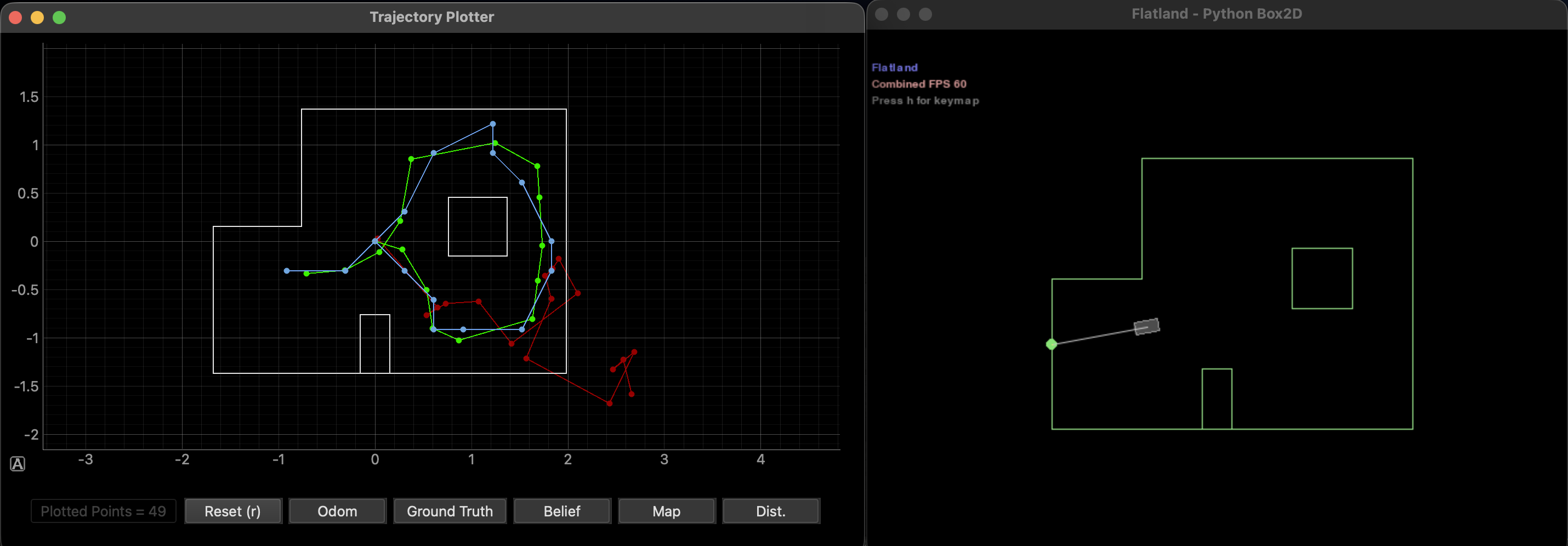
Lab 11 simulation run — Bayes filter belief tracks ground truth

Simulation verification: Bayes filter belief (blue) closely follows ground truth (green), while odometry (red) drifts significantly.

3. Real Robot: Observation Pipeline

The core addition for Lab 11 is implementing $RealRobot.perform_observation_loop()$ inside $lab11_real.ipynb$ . The method:

Subscribes to BLE notifications, sends $START_SCAN$ to the Artemis, and waits for the full 360° scan to complete.
Requests data via $GET_SCAN_DATA$ and parses packets of the form $A:<angle_deg>|D:<dist_m>$ .
Requires exactly 18 readings; raises a $RuntimeError$ if the scan is incomplete (protects against requesting data before the robot finishes turning).
Reorders ranges for clockwise physical rotation: the mapper expects counter-clockwise bearings $[0°, 20°, \dots, 340°]$ , so index 0 is kept at 0° and indices 1–17 are reversed.

The same step-and-scan turning mechanism from the wall-mapping lab was reused here.

def perform_observation_loop(self, rot_vel=120):
    # BLE notify, START_SCAN, time.sleep to allow full scan to finish
    # GET_SCAN_DATA, wait until len(raw_packets) >= expected_obs
    # Parse A:|D: packets into angles_deg, dists_m

    if len(dists_m) != expected_obs:
        raise RuntimeError(
            f"Incomplete scan data: expected {expected_obs}, got {len(dists_m)}"
        )

    # Robot rotates CW; mapper expects CCW order [0, +20, ..., +340]
    dists_ccw   = [dists_m[0]] + list(dists_m[1:][::-1])
    angles_ccw  = [angles_deg[0]] + list(angles_deg[1:][::-1])

    sensor_ranges   = np.array(dists_ccw)[np.newaxis].T
    sensor_bearings = np.array(angles_ccw)[np.newaxis].T
    return sensor_ranges, sensor_bearings

4. Configuration Tuning

$sensor_sigma$ in $config/world.yaml$ was tuned to balance sensitivity to real ToF noise versus over-smoothing the likelihood. A larger value makes the update more tolerant of outlier readings and occasional failed measurements. After experimentation, $sensor_sigma = 0.4$ performed well across most runs. All experiments used 18 observations and $ray_tracing_length: 6$ m by default, except at (5, −3) where targeted adjustments were explored.

mapper: observations_count: 18 ray_tracing_length: 6 localization: sensor_sigma: 0.4

Firmware note: The VL53L1X was configured in short distance mode in the Lab 11 Arduino sketch. This maximizes sample rate but can limit usable range on long return paths. A sufficiently long $time.sleep$ after $START_SCAN$ ensures all 18 packets are logged before $GET_SCAN_DATA$ is called.

5. Marked Poses and Results

The robot was placed at four marked poses on the course map, each with a nominal heading of 0°. Ground truth is measured in feet (1 ft ≈ 0.3048 m). For each pose, the filter was initialized with a uniform belief, one observation loop was performed, and $loc.update_step()$ was run to compute the posterior.

Pose (ft)	Ground Truth (m)	Peak Belief (x, y, θ°)	Peak Prob	Notes
(−3, −2)	(−0.914, −0.610)	(−0.610, 0.000, 50.0°)	0.950	Clean result — geometrically distinct corner
(0, 3)	(0.000, 0.914)	(−0.400, 0.600, 50.0°)	0.800	Good match — open-center landmark (see plot)
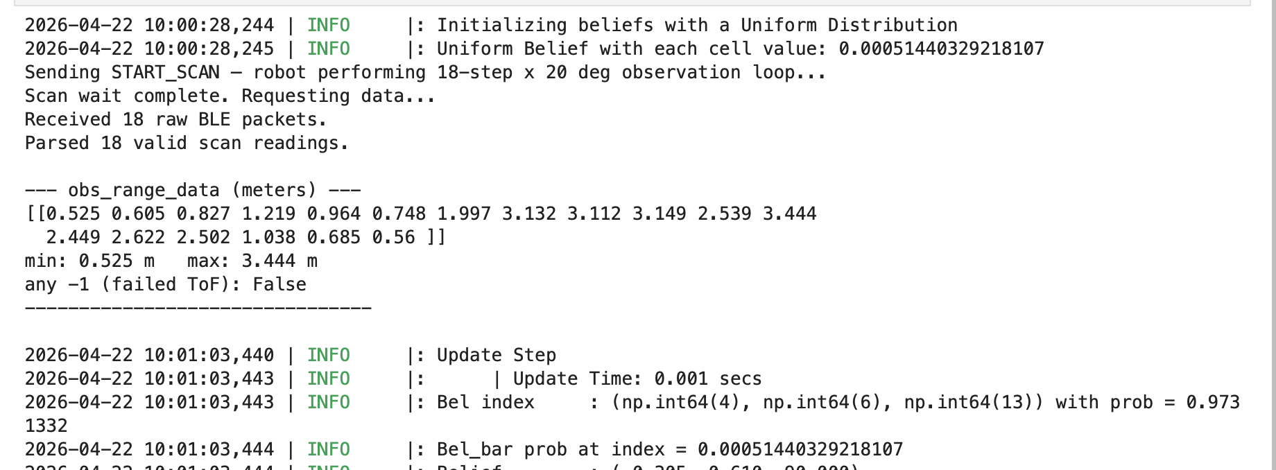
(5, −3)	(1.524, −0.914)	Off-true cell		Hardest pose — perceptual aliasing (see §6)
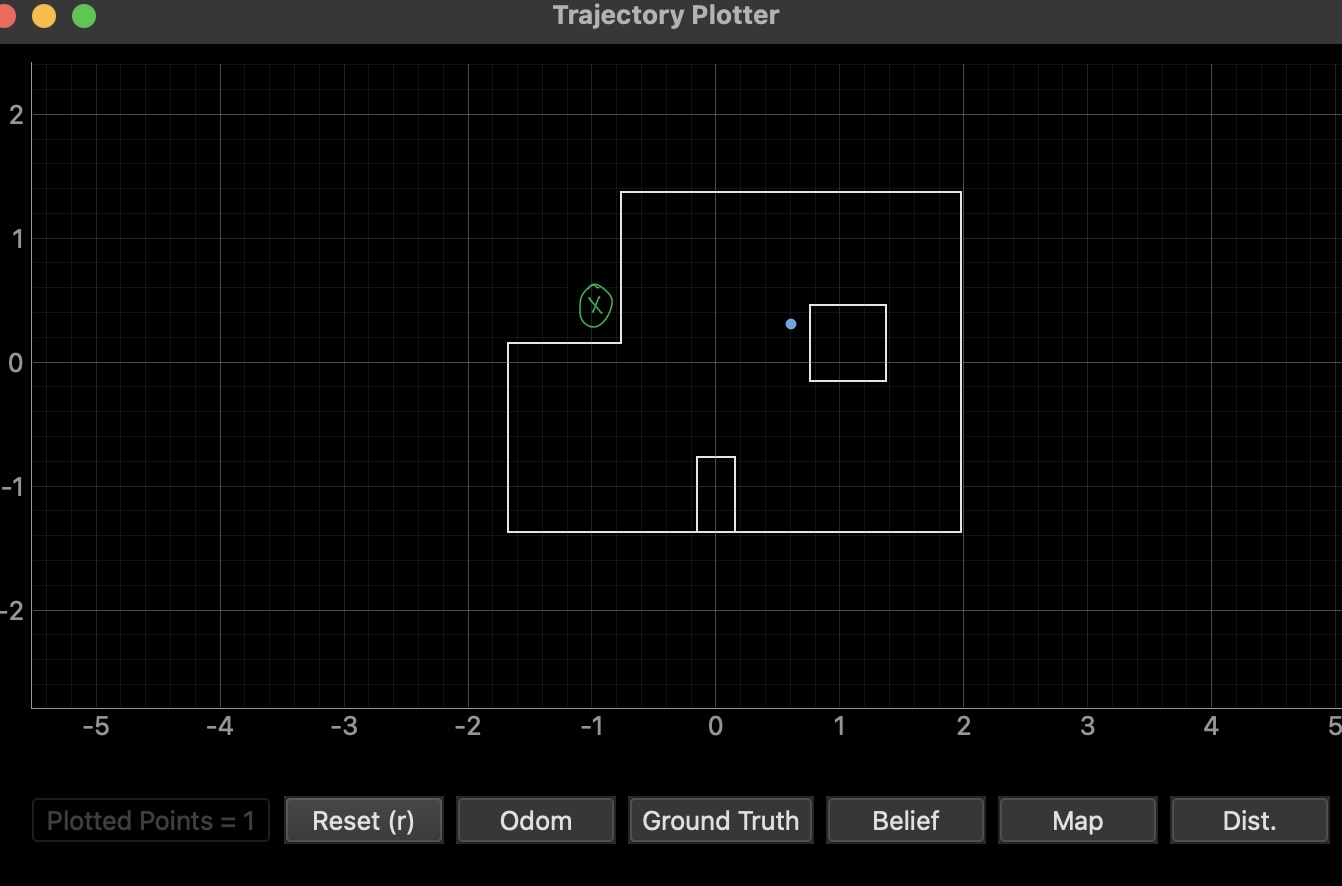
(5, 3)	(1.524, 0.914)	(1.219, 0.914, 150.0°)	0.624	Solid result — corner with distinct wall geometry

Pose (−3, −2) ft

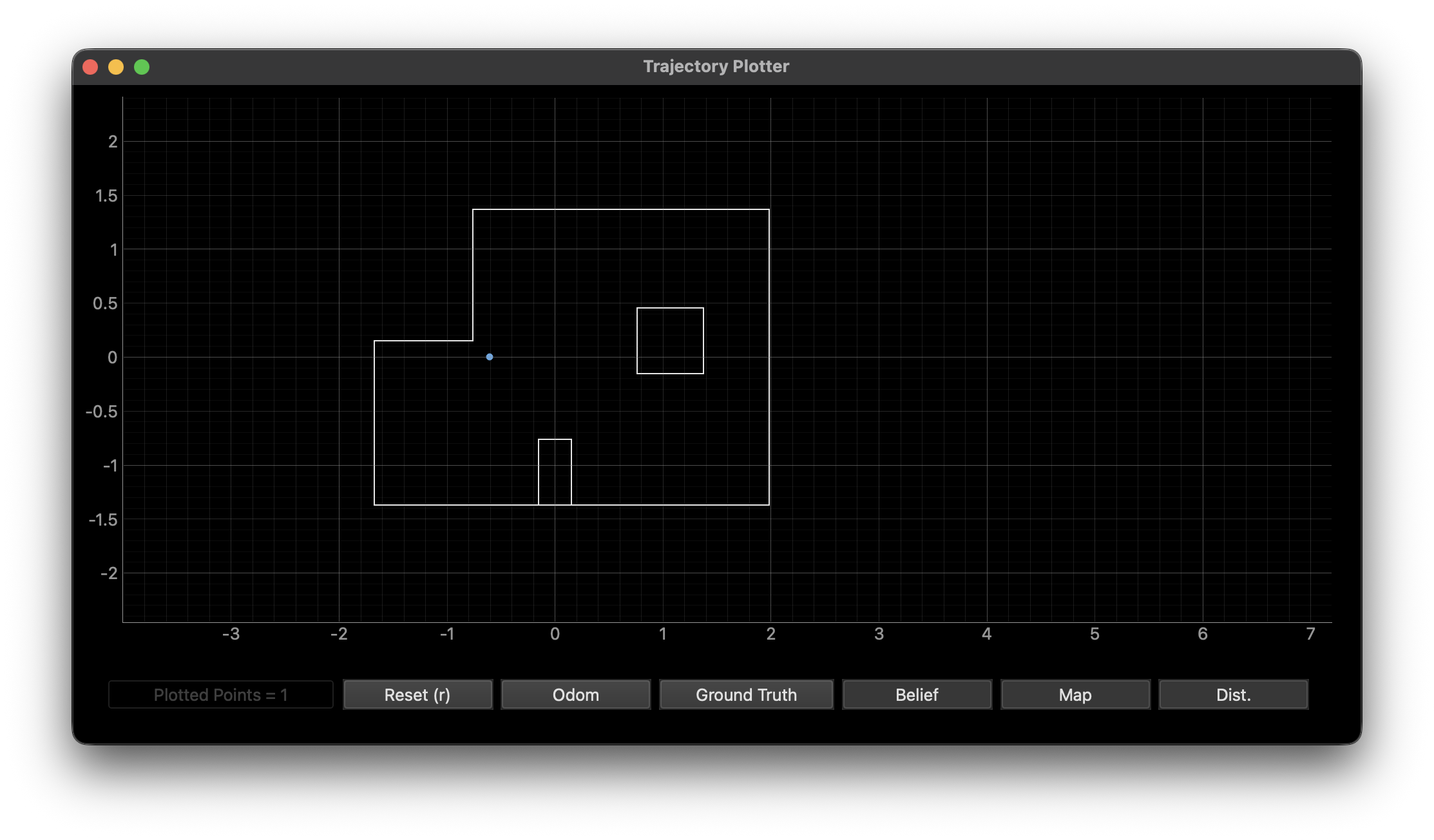
Belief plot for pose (-3, -2) — simulator view

Simulator view — belief after update step.

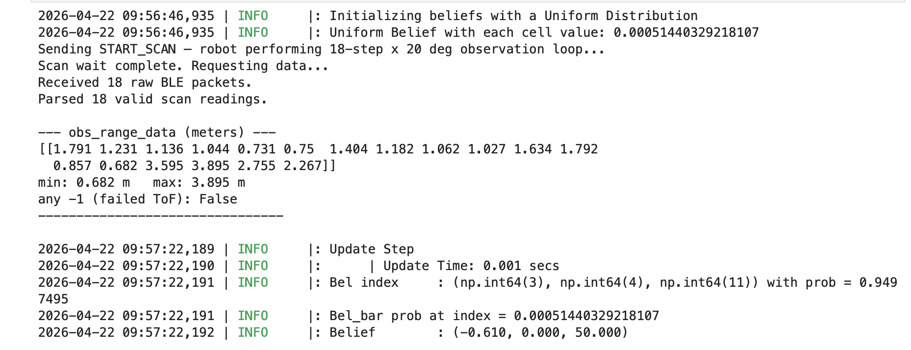
Belief plot for pose (-3, -2) — Python notebook output

Notebook posterior — peak at (−0.610, 0.000, 50°), p=0.950.

This geometrically distinct corner produced a clean, high-confidence estimate (p = 0.950). The 18-ray scan provides a unique angular signature: two nearby walls at perpendicular angles create a range profile that is hard to replicate elsewhere on the map, so the update step converges strongly to the correct cell.

Pose (0, 3) ft

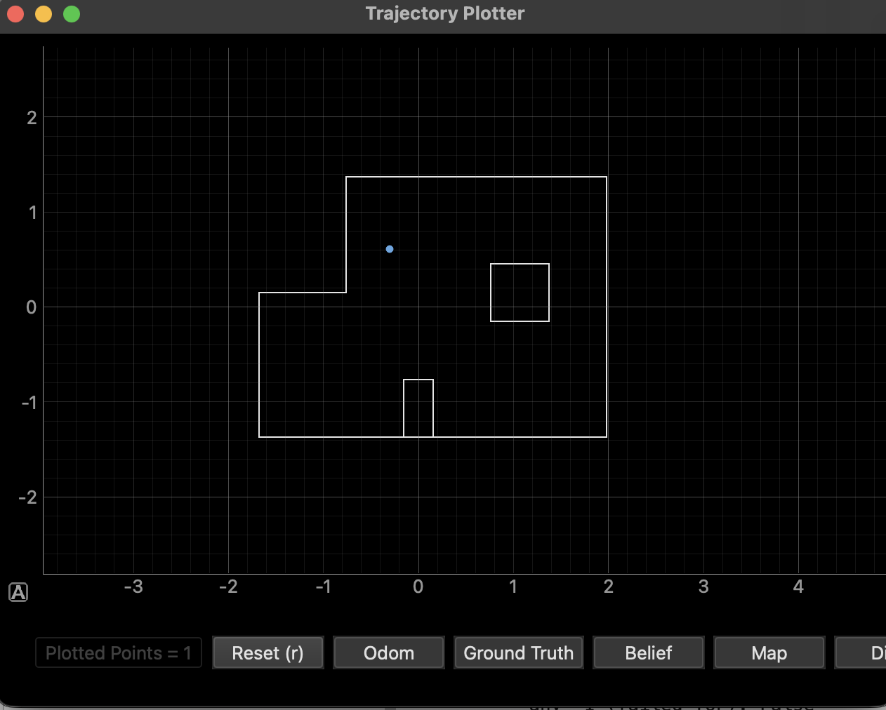
Belief plot for pose (0, 3) — simulator view

Simulator view — belief concentration after update.

Belief plot for pose (0, 3) — Python notebook output

Notebook posterior — update step narrows belief to the correct region.

A near-center position with good angular diversity — the robot can "see" all four walls from this location, giving the 18-ray scan enough discriminative information to converge to the correct cell.

Pose (5, −3) ft

Belief plot for (5, −3) — the MAP estimate lands off-true spot.

This pose produced the weakest localization result. The outer-wall geometry near (5, −3) is not unique enough at 20° scan resolution — a nearby cell with similar ray-cast distances can outscore the ground-truth cell after the update. See §6 for a full breakdown.

Pose (5, 3) ft

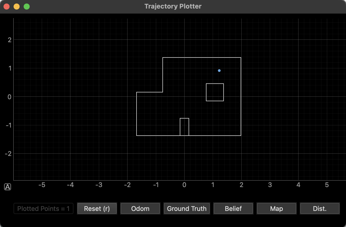
Belief plot for pose (5, 3) — simulator view

Simulator view — belief after update step.

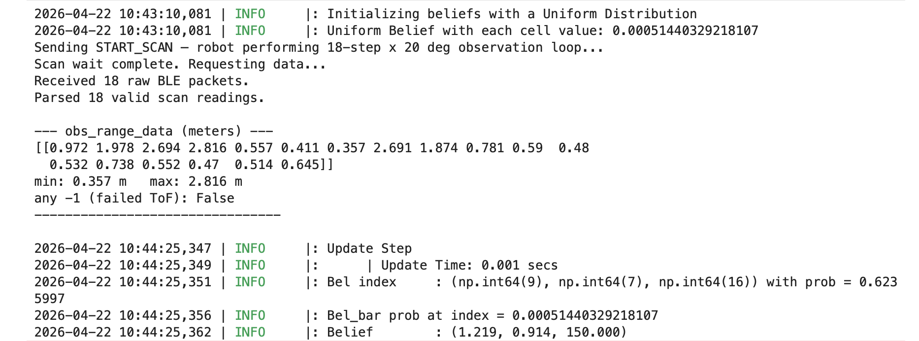
Belief plot for pose (5, 3) — Python notebook output

Notebook posterior — peak at (1.219, 0.914, 150°), p = 0.624.

The corner geometry at (5, 3) provides discriminative ray casts — two short wall distances at roughly perpendicular angles give the filter enough information to pinpoint the correct cell with a peak probability of 0.624. The lower confidence compared to (−3, −2) likely reflects slightly more open sight lines on one side, which allows a small amount of probability mass to spread to adjacent cells.

6. Discussion: Why (5, −3) Was the Hardest

At (5, −3), the maximum a posteriori cell sometimes landed in a visually "similar" pocket near an outer wall( the green x in 5,-3 in image above). From the robot's ToF view, a wrong $(x, y, θ)$ could still produce a passable match to the cached ray cast — classic perceptual aliasing at a coarse 20° scan resolution.

Several experiments were run to improve this result:

Increasing $observations_count$ brought the estimate closer, but not exact.
Reducing $ray_tracing_length$ for targeted runs had a similar effect.

Root causes:

1. Sparse angular sampling (18 directions, 20° steps): parallel outer walls at comparable ranges look alike from different positions.

2. Sensor limits: Short distance mode truncates or fails on the farthest wall returns, so certain beams carry less discriminative information and inter-cell similarity increases.

3. Invalid readings: ToF failures logged as $-1$ down-weight the correct cell because the likelihood model doesn't explicitly handle outliers.

7. Takeaways

The update-only Bayes filter with a uniform prior is highly sensitive to how well the observation vector is aligned with the map (rotation direction, beam ordering, heading at time of scan).
Tuning $sensor_sigma$ on hardware is necessary; a single simulation-derived value is rarely transferable directly.
A single difficult pose is expected in environments with degenerate symmetry; finer angular resolution, more beams, or explicit outlier handling would be the natural next steps.

AI usage: AI was used to build this site and to help format and structure the lab writeup.